Theory Learner (TL) is a prototype system for learning progressively better executable, empirically evaluable theories of the physical world. It models the world as an unknown state-transition function and the learner as an embedded subsystem within that world.
The central objective is to retain theory updates only when they increase validated empirical agreement with the unknown state-transition function, evaluated on a finite ledger of forward-chaining comparison instances. The formulation avoids stochastic-law assumptions and does not treat learning as an inductive update rule. From this selection problem, TL derives a second objective: to maximize the physical rate of total agreement growth. This objective is used to refine a heuristic function, instantiated in the current prototype as a language-model policy.
In the current prototype (TLv1), the language-model policy drives theory proposal and observation attempts. TLv1 records provenance across the computations that lead to successfully observed outcomes, approximated through bytecode-level tracing of dynamically executed theory, memory, and conversation files. When a candidate theory update is validated, credit is propagated backward through that ancestry so earlier contributing artifacts receive reward.
This essay presents the formal model and a small-scale implementation that iteratively improves, by selection, an executable theory by performing a sequence of crucial experiments. The system is proposed as a possible end-to-end formalization of scientific learning that discovers better theories of the physical world through conjecture, empirical test, and selective retention.
Brief Introduction
The Theory Learner (TL) prototype is organized around four guiding ideas.
Learning lacks a universally accepted formal definition, and it may be possible to formulate one that is more general and less assumption-heavy than the account given by statistical learning theory.
Science, as currently practiced, may be understood as an informal approximation to a process that is, in principle, formally definable and automatable by a universal computing device operating by finite means (Deutsch 1985).
Because science is carried out by physically instantiated learners, its formalization should be grounded in features of the physical world rather than treated as a purely mathematical abstraction.
This formalization will sharpen a Critical Rationalist conception of scientific learning rather than rely on inductive primitives (K. R. Popper 1963; Deutsch 2011, 2012; K. Popper and Miller 1983). In particular, it will avoid unnecessary assumptions such as fundamental randomness (Deutsch 2016) while keeping constraints on the hypothesis space as weak as possible.
TL is a prototype implementation of this general picture. For philosophical background and discussion of related automated learning systems, see Appendix A and Appendix B.
The rest of the essay has two parts: Theory develops the formal model; Implementation describes how TL instantiates it.
Theory Overview
TL separates selection-based theory improvement from algorithmic refinement of the heuristic function \(c\). A theory is a computable program \(f\) that maps partial observations of world state \(x_t\) from a sensor interface \(s\) to predictions of subsequent observations. The heuristic function \(c\) proposes candidate revisions to \(f\), while an evaluator \(h\) determines whether a proposed revision increases observed agreement with \(w\).
Given an evaluation context \(E\), \(c\) proposes a candidate \(f'\) by structured edits to the incumbent \(f\). The evaluator \(h\) promotes \(f'\) only if it yields a strict net increase in empirical agreement on a fixed comparison ledger consisting of previously validated target events together with newly committed forward-chaining instances from \(E\).
When validated progress triggers reward, TL traces backward from the credited roots through the provenance directed acyclic graph (DAG) of the computation that produced that outcome and distributes credit across the contributing ancestry. Artifacts generated by \(c\) that lie on rewarded provenance paths pass credit backward to the earlier outputs of \(c\) that generated them. TL uses the resulting weights on outputs attributable to \(c\) to construct offline updates, biasing \(c\) toward generating the kinds of executable artifacts that help produce theory improvements validated by \(h\), in proportion to how much they contributed within the rewarded provenance.
Implementation Overview
This section describes a working implementation of the TL objective: a system that proposes edits to an executable theory, evaluates those edits on forward-chaining observation instances, promotes only validated improvements, and uses provenance-based credit assignment to bias later updates of the refined heuristic function \(c\). In the implemented Theory Learner version 1 (TLv1), \(c\) is instantiated as a tool-augmented GPT-OSS-20B policy, and the implementation discussion points to companion artifact pages covering rewarded observations, evaluator calibration, and successive training checkpoints.
The implementation is built around two architectural commitments:
All theory, memory, and conversation text is stored as versioned, editable state (piece tables), so these objects can be revised while preserving reconstructable lineage.
All system-managed artifacts are provenance-tracked, so external inputs, outputs attributable to \(c\), tool results, and compute results from managed Python files can be traced in a dependency graph for auditability and credit assignment.
In TLv1, this provenance-first ideal is approximated through tracked tool and model interactions together with bytecode-level tracing over dynamically executed theory and memory files.
Theory
This section gives a minimal, representation-agnostic formal model of TL’s learning loop. It specifies how an embedded learner constructs committed forward-chaining comparison instances from ordered observations, evaluates competing theories on a fixed comparison ledger, validates improvements, and uses successful outcomes to update the refined heuristic that proposed them. The primary optimization problem is to expand the domain over which the theory function \(f\) empirically agrees with the world process \(w\). In the formalism below, this is witnessed locally as strict growth in validated empirical agreement on that ledger. Because the learner is physically embedded in \(w\), TL also induces a secondary optimization problem: to maximize the physical rate of that growth. Notation and the notation-to-system mapping are collected in Appendix C.
The learner’s primitive input is an ordered stream of partial observations \((x_t)\) arising from an underlying sequence of full world states \((X_t)\), where \(X_t\) includes the learner itself.
The world evolves according to an unknown state-transition function \(w\), and the learner receives only a partial view of each world state through a sensor map \(s\): \[
X_{t+1} = w(X_t),
\qquad
x_t = s(X_t).
\]
Let \(\mathcal{X}\) be the space of full world states and \(\mathcal{O}\) the space of partial observations, so that \(X_t \in \mathcal{X}\), \(x_t \in \mathcal{O}\), \(w : \mathcal{X} \to \mathcal{X}\), and \(s : \mathcal{X} \to \mathcal{O}\). The observation stream is a trajectory in \(\Omega := \mathcal{O}^{\mathbb{N}}\), equipped with the \(\sigma\)-algebra generated by finite-prefix cylinder events. No probability law is assumed.
The index \(t\) marks only successor order in the world and observation stream; no metric or fundamental time parameter is assumed. Both \(w\) and \(s\) are treated as deterministic. The learner need not observe the full state \(X_t\): the comparison objects introduced below are constructed from the ordered observation stream alone.
Primary Optimization Problem: Selecting Theories to Expand Validated Empirical Agreement
This section defines the fixed comparison ledger, the empirical agreement score on that ledger, and the promotion rule that selects between incumbent and candidate theories.
The current theory is represented as an executable program \(f\), treated here as a total function \[
f : \mathcal{O}^{*} \to \mathcal{O},
\] where \(\mathcal{O}^{*}\) denotes finite ordered tuples of observations.
Evaluation is performed on a fixed comparison ledger of forward-chaining instances. It consists of previously validated target events carried forward from earlier successful promotions together with newly committed instances whose contexts are fixed before their targets are observed and whose targets are supplied by later incoming sensor data.
Instance Ledger \(\Omega_E\)
Let \[
E = (x_1, \dots, x_n)
\] be the current finite evaluation window, listed in sequence order. Within this window, use \(i\) for local position; global stream indices are suppressed for compactness.
Construct the newly committed forward-chaining instances in three steps. First, choose a set of target positions \[
I \subseteq \{2, \dots, n\}.
\]
In the present formalism, each candidate-theory evaluation step is allowed to commit at most one new target event. Accordingly, restrict \[
|I| \le 1.
\] This single-target restriction ensures that any one candidate update can contribute at most one newly validated forward-chaining instance at that step; larger net gains require a chain of distinct updated theories across successive evaluation steps.
Second, for each \(i \in I\), choose a non-anticipating context \[
g(i) = (x_{j_1}, \dots, x_{j_m}),
\qquad
1 \le j_1 < \cdots < j_m < i,
\] so each context is an ordered tuple of observations drawn only from positions earlier than its target. This non-anticipation constraint ensures that theory evaluation is restricted to forward-chaining transformations from earlier partial states to later ones, mirroring the successor-ordered structure induced by the world transition function under partial observation rather than allowing arbitrary retrospective fits over the evaluation window.
Third, for each \(i \in I\), let \(\lambda_i\) denote the newly committed ledger element with fixed target \[
x(\lambda_i)=x_i
\qquad\text{and}\qquad
\mathcal{C}(\lambda_i)=\{g(i)\}.
\] Define the newly committed instance set by \[
\Omega_E^{\mathrm{new}} := \{\lambda_i : i \in I\}.
\]
Let \(\Omega_E^{\mathrm{old}}\) denote the previously validated target events carried forward from earlier successful promotions. Each carried-forward element likewise fixes a target \(x(\lambda)\) together with an admissible replay-context set \(\mathcal{C}(\lambda)\), where every context in \(\mathcal{C}(\lambda)\) is an ordered tuple of observations drawn only from positions strictly earlier than that target. By construction, only those previously validated elements on which the current incumbent still succeeds under admissible replay are retained in \(\Omega_E^{\mathrm{old}}\). The fixed comparison ledger at the current evaluation step is then \[
\Omega_E := \Omega_E^{\mathrm{old}} \cup \Omega_E^{\mathrm{new}}.
\]
Each ledger element therefore fixes a target observation together with an admissible replay-context set. Newly committed elements have singleton admissible sets \(\mathcal{C}(\lambda_i)=\{g(i)\}\), while replayed validated elements may have larger admissible sets. Thus \(f'\) is tested against the same validated target events as the incumbent, even when replay uses a different admissible context.
Empirical Agreement Score \(T_{\Omega_E}\)
On \(\Omega_E\), use the discrete \(\sigma\)-algebra and counting measure \(\mu_E\).
For a ledger element \(\lambda \in \Omega_E\), let \(x(\lambda)\) denote its fixed target observation and let \(\mathcal{C}(\lambda)\) denote its admissible set of replay contexts. Define the empirical agreement score on the fixed comparison ledger by counting the ledger elements for which the theory succeeds on at least one admissible replay context:
This counts the ledger elements for which the theory succeeds on at least one admissible replay context. Here \(\gamma\) ranges over admissible replay contexts in \(\mathcal{C}(\lambda)\), and \(\mathrm{Eq}(f(\gamma), x(\lambda))\) denotes equivalence between the replayed output and the fixed target observation associated with \(\lambda \in \Omega_E\).
Promotion under \(T_{\Omega_E}\)
Promotion compares the incumbent theory \(f\) and a candidate update \(f'\) on the same fixed comparison ledger \(\Omega_E\). By construction, every element of \(\Omega_E^{\mathrm{old}}\) is a previously validated instance on which the current incumbent still succeeds; instances on which the incumbent fails are not carried forward.
Promotion requires a strict net gain in empirical agreement: \[
T_{\Omega_E}(f') > T_{\Omega_E}(f).
\] Moreover, on the carried-forward old instances the candidate cannot do better than the incumbent: \[
T_{\Omega_E^{\mathrm{old}}}(f') \le T_{\Omega_E^{\mathrm{old}}}(f)=|\Omega_E^{\mathrm{old}}|.
\] So any strict gain over the incumbent must come from newly committed instances in \(\Omega_E^{\mathrm{new}}\). Agreement on old validated targets only preserves the candidate’s margin, while regressions on them reduce it.
At a given evaluation step, let \(\Omega_E\) be the fixed comparison ledger, let \(f\) be the previously accepted theory, let \(f'\) be a proposed update, and define \(F := \{f, f'\}\). In the pairwise setting, the evaluator is \[
h(\Omega_E, F) =
\begin{cases}
f' & \text{if } T_{\Omega_E}(f') > T_{\Omega_E}(f),\\
f & \text{otherwise.}
\end{cases}
\] Define the associated success signal by \[
\text{success}(\Omega_E, f', f)
:= \mathbf{I}\!\bigl(h(\Omega_E, F)=f'\bigr).
\] Then a learning step occurs exactly when \(\text{success}(\Omega_E, f', f)=1\).
As later targets are observed, newly committed instances may be added to later comparison ledgers. Thus, a candidate can fail promotion even after getting a new target right if it regresses on enough carried-forward old instances to offset that gain.
Under the single-target restriction \(|I|\le 1\), each successful step can contribute at most one newly validated target event. Larger net gains require a sequence of successive promotions across multiple evaluation steps. Formally, if \[
f^{(0)}, f^{(1)}, \dots, f^{(m)}
\] is a sequence of accepted theories such that, at step \(k\), the evaluator promotes \(f^{(k+1)}\) over \(f^{(k)}\) on that step’s fixed comparison ledger, then the validated gains retained by earlier promotions can accumulate across the sequence. Thus a later accepted theory may eventually exceed a much earlier incumbent even when no single candidate update would have achieved that net gain in one step.
Secondary Optimization Problem: Refining \(c\)
Objective and Intuition
TL’s secondary optimization problem is to maximize the rate at which total agreement between the theory function \(f\) and the world process \(w\) grows. An instantiated learner cannot measure this objective directly as it cannot observe either a theory’s absolute agreement with the world or the rate of verifiable theory updates relative to the full sequence of world-state updates. Therefore, TL approaches the objective indirectly.
The function \(c\) revises \(f \mapsto f'\), selects computations and predictive contexts, and submits them to \(h\) for evaluation. It is reinforced when its choices contribute to later successful evaluations that promote a candidate theory over the incumbent. In this way, the secondary objective refines the search procedure without restricting the space of candidate theories considered under the primary objective.
The setup bootstraps as the accepted theory \(f\) becomes a better approximation to the world process \(w\) and more of \(c\)’s future choices can be guided by explicit theory content rather than open-ended search. In turn, successful theory improvements generate better-targeted update records for refining \(c\), so improvements in \(f\) and in \(c\) can reinforce one another across many learning steps.
Each propose-evaluate-promote cycle in TL is itself a physical process within the world. Because all symbolic inputs to and outputs from \(c\) are provenance-trackable within TL up to the sensor boundary, the system can identify deterministically which outputs of \(c\) directly or indirectly contribute to later theory promotions. Therefore, outputs that contribute to validated agreement gains are reinforced more often when they help produce them after fewer intervening interaction steps. The induced pressure on \(c\) is consequently toward generating outputs that increase the rate of validated agreement growth in world order, without requiring a privileged definition of time.
The total agreement domain between a theory and the world process may be infinite. TL instead uses a provenance-based proxy: when a validated gain releases reward, that reward is assigned to the computation that produced the rewarded root and then propagated backward through its provenance DAG until it reaches artifacts attributable to \(c\). This payout is hierarchical, because reward is assigned first within a local rewarded slice before it is passed recursively across provenance boundaries into deeper computational ancestries. The number of recursive crossings provides a simple notion of how indirect an output of \(c\)’s contribution was to the credited outcome. This does not identify the full agreement domain of an artifact with respect to \(w\); rather, it provides an operational approximation that preferentially reinforces outputs of \(c\) that repeatedly participate in computations culminating in validated theory improvement. If an artifact’s relative presence in the computational provenance of successfully validated agreement points tracks, even approximately, the relative extent of its agreement domain in the extensional structure of \(w\), then this payout procedure will tend to shape \(c\) toward generating and validating artifacts with larger implicit agreement domains.
Local Promotion and Reward Release
Promotion and reward release are distinct. Promotion is local under \(h\), while reward release depends on whether the newly accepted theory sets a strict new record relative to the previous reward-generating theory.
At each evaluation step, the candidate theory \(f'\) is compared with a previously promoted theory \(f\) using that step’s ledger \(\Omega_E\). Equivalently, \[
h(\Omega_E,\{f,f'\}) = f'
\iff
T_{\Omega_E}(f') > T_{\Omega_E}(f).
\]
Each accepted promotion \(f \mapsto f'\) also defines the provenance-addressable roots associated with the target events validated at that step. Let \[
\mathcal{N}(f,f')
\] denote this step-local root set.
For any single comparison under \(h\), \(\Omega_E\) is fixed. Across successive evaluations, however, successful promotions together with newly observed target events can enlarge the ledger used at later steps. Earlier promoted theories are replayed on the current ledger.
Reward is issued by a stricter rule than local promotion. Let \(\mathcal{H}_{\mathrm{prom}}\) be the set of previously promoted theories. On the current ledger \(\Omega_E\), define the previous record by \[
T_{\Omega_E}^{\max}
:=
\max_{\tilde f \in \mathcal{H}_{\mathrm{prom}}} T_{\Omega_E}(\tilde f).
\] Then the newly accepted theory releases unit reward only if it sets a strict new record on the current ledger: \[
R := \mathbf{I}\!\bigl(T_{\Omega_E}(f') > T_{\Omega_E}^{\max}\bigr)
\in \{0,1\}.
\]
Thus a theory may be promoted locally without releasing reward. Under \(|I|\le 1\), larger increases in the record value of \(T_{\Omega_E}\) can accordingly arise only across a chain of accepted promotions.
If the newly accepted theory sets a new record, let \[
\mathcal{R}
\] be the set of roots whose validated target events account for the increment beyond the previous record on the current ledger. This credited set can include roots introduced by earlier accepted promotions whose gains were necessary for the new record. The released unit reward is then split uniformly across those roots: \[
R_r := \frac{1}{|\mathcal{R}|},
\qquad r \in \mathcal{R}.
\]
This separates local theory selection from reward release. Roots are defined locally when \(h\) promotes a candidate theory, but payout is triggered only when the accepted sequence raises the record value of validated agreement measured on the current ledger.
Provenance-Based Credit Assignment
The heuristic function \(c\) should be updated so that its outputs compete for influence only through their deterministic empirical contribution to successful rewarded learning. The aim is to avoid extraneous bias in credit assignment.
The computational provenance system in TL abstracts the read-write history of the underlying computation: each tracked write receives a stable sequence identifier together with the read identifiers that contributed to the machine state at that step.
When TL assigns payout to a reward-generating artifact (root), it constructs a provenance DAG from that write identifier and its recorded read-state ancestry. TLv1 uses an explicit high-level approximation that is sufficient for deterministic, auditable payout.
Within this provenance DAG, absorbing artifacts are the written artifacts directly attributable to \(c\); only these may retain reward. Relevant non-absorbing artifacts are those that lie on some provenance path from an absorbing artifact to the rewarded root.
For each credited root \(r\in\mathcal{R}\), the payout rule propagates the share \(R_r\) backward through this relevant ancestry, producing terminal weights over upstream artifacts attributable to \(c\). Absorbing artifacts retain terminal weight, while non-absorbing artifacts route reward recursively into earlier history. This organization is intended to make payout deterministic, hierarchical, specific to empirically useful contributions, and compatible with termination and conservation.
The rule below is presented as a provisional replacement candidate for the original implemented TLv1 payout logic, intended to capture these invariances more directly.
Proposed Payout Rule
The implemented TLv1 payout algorithm appears more complicated and more biased than necessary. In particular, defining the computational “spine” exclusively from artifacts directly attributable to \(c\) is somewhat arbitrary, grouping artifacts with shared dependencies may concentrate reward in a gameable way, and permitting recursive payout to spine artifacts may introduce a primacy bias. The candidate formulation below is intended as a simpler, less gameable replacement for future training. This is my favored version of the payout algorithm to date.
At a high level, the construction has four stages: identify the artifacts in the credited root’s provenance that lie on a path from an absorbing artifact to \(r\); construct a single spine through that relevant ancestry by backtracing the relevant parent with the greatest stable sequence identifier at each step; collect the off-spine boundary artifacts and distribute incoming reward uniformly across the resulting recipient artifact set, recursing only at non-absorbing boundary artifacts; and aggregate the terminal weights \(W_r(a)\) into weighted update records \(\mathcal{D}\) for improving \(c\).
Relevant ancestry
Let \(G = (V, E_G)\) be the provenance DAG of the rewarded root \(r\).
Let \(\operatorname{AttrToC}(v)\) indicate that artifact \(v\) is directly attributable to \(c\).
Let \[
A_G := \{\, a \in V \mid \operatorname{AttrToC}(a)=1 \,\}
\] be the set of absorbing artifacts in \(G\).
Let \[
V_r^{\mathrm{rel}} := \{\, v \in V \mid \exists a \in A_G \text{ such that } a \to^{*} v \to^{*} r \,\}
\] be the set of payout-relevant artifacts, lying on some provenance path from an absorbing artifact to \(r\).
Spine construction
For any artifact \(v \in V_r^{\mathrm{rel}}\), let \[
P(v) = \{\, u \in V_r^{\mathrm{rel}} \mid (u,v) \in E_G \,\}
\] denote its relevant parent set, and let \(\operatorname{ord}(v)\) denote the total order of \(v\) induced by its stable sequence identifier.
Define the spine of \(r\) by sequence-order backtracking over \(V_r^{\mathrm{rel}}\).
Set \[
v_0 = r.
\]
If \(P(v_i) \neq \varnothing\), define \[
v_{i+1} = \arg\max_{u \in P(v_i)} \operatorname{ord}(u),
\] and continue until no relevant parent remains.
This produces a chain from root to oldest ancestor: \[
(v_0, v_1, \dots, v_k).
\]
Reverse it to obtain the main spine: \[
S(r) = (v_k, \dots, v_0).
\]
Absorbing artifacts on the spine
Define the absorbing spine set \[
A(r) = \{\, s \in S(r) \mid \operatorname{AttrToC}(s)=1 \,\}.
\]
These are the only spine artifacts that hold the reward they receive.
Boundary artifacts
Define the boundary set of the spine as the set of relevant parent artifacts attached to the spine that are not themselves in the spine: \[
B(r) = \left( \bigcup_{s \in S(r)} P(s) \right) \setminus S(r).
\]
Because \(B(r)\) is a set, repeated occurrences of the same artifact are counted only once.
Recipient artifact set
Define the recipient artifact set of the root by \[
\Gamma(r) = A(r) \cup B(r).
\]
The terminal artifact reached by backtracing the spine has no relevant parent and lies in \(A(r)\), so \(\Gamma(r)\neq\varnothing\). If reward entering artifact \(r\) is \(R_{\mathrm{in}}(r)\), define the per-artifact share \[
\sigma(r) = \frac{R_{\mathrm{in}}(r)}{|\Gamma(r)|}.
\]
Recursive payout
A recursive payout call is parameterized by a current root \(q\) and incoming reward \(R_{\mathrm{in}}(q)\). Reapply the construction above with \(q\) in place of \(r\) to obtain the corresponding relevant ancestry, spine, boundary, and recipient set \(\Gamma(q)\), and define \[
\sigma(q) = \frac{R_{\mathrm{in}}(q)}{|\Gamma(q)|}.
\]
For each recipient artifact \(u \in \Gamma(q)\):
if \(\operatorname{AttrToC}(u)=1\), assign terminal reward \(\sigma(q)\) to \(u\);
otherwise, start a new payout call at root \(u\) with incoming reward \(R_{\mathrm{in}}(u):=\sigma(q)\).
For each absorbing artifact \(a \in A_G\), let \(W_q(a)\) denote the total terminal reward assigned to \(a\) by the payout call rooted at \(q\). Equivalently, \[
W_q(a) =
\sum_{u \in \Gamma(q)}
\begin{cases}
\sigma(q) & \text{if } u = a \text{ and } \operatorname{AttrToC}(u)=1, \\
W_u(a) & \text{if } \operatorname{AttrToC}(u)=0, \\
0 & \text{otherwise}.
\end{cases}
\]
For the original credited root \(r\), the terminal reward distribution is therefore \(a \mapsto W_r(a)\).
Termination is guaranteed because each recursive call moves to a strict ancestor in the finite provenance DAG. Reward is conserved because each call partitions its full incoming reward uniformly across \(\Gamma(q)\).
Weighted Update Records \(\mathcal{D}\)
For the payout rule above, let \[
A_r^{\star} := \{\, a \in A_G \mid W_r(a) > 0 \,\}
\] denote the set of terminal absorbing artifacts attributable to \(c\) that receive positive weight under recursive payout from root \(r\). Define \[
\omega_r(a) := W_r(a),
\qquad a \in A_r^{\star}.
\]
Let \(\rho(a)\) denote the abstract update record for artifact \(a\), containing the locally logged material used to update \(c\) toward producing \(a\).
The theory does not assume any particular representation of \(c\) or any specific update mechanism. It requires only that larger weights \(\omega(a)\) correspond to stronger reinforcement of the choices encoded by \(\rho(a)\).
The core equations for this theory-side payout rule are collected in Appendix C for reference.
Implementation
Theory Learner version 1 (TLv1) is a prototype that instantiates the abstractions defined above.
In this prototype, \(c\) is a tool-augmented language-model policy, \(f\) is versioned executable theory modules, \(s\) is logged responses from a human ‘tutor’ to \(c\)-generated contexts, and \(h\) is a conservative observation pipeline. TLv1 realizes provenance and credit assignment through piece tables (representing conversation, memory, and theory state) runtime object dependency tracking. Appendix C provides notation-to-system mapping.
One important implementation deviation, alongside the payout variation already noted, is that empirical agreement is judged using a single conditional-loss proxy on sensor data. A candidate theory is accepted only when conditioning on its output lowers conditional sequence loss on the sensor_data enough to place the resulting score above an adaptive cutoff calibrated from the observed separation between materially improving and non-improving cases.
When a step succeeds, the system promotes the candidate theory and runs provenance-based credit assignment rooted at the credited outcome artifact. Weights on outputs attributable to \(c\) are later used to weight offline supervised fine-tuning (SFT) updates to \(c\). Curated companion records are collected on the Artifacts page.
Learning Loop Overview
Persistent State and Tracked Artifacts
Because TL learns by modifying theory, memory, and conversation text, it must store that text as editable state with stable artifact identity. In TLv1, mutable text lives in piece tables, and each piece-table segment carries a definition ID (def_id). This is a system-assigned globally unique identifier that also names a node in the provenance graph.
The key persisted structures at this stage are the piece tables themselves, an append-only edit log (tx_begin/edit/tx_commit) for replay and hash-based reproducibility, and a provenance DAG keyed by def_id.
Edits create or reuse definition artifacts and write those IDs into piece-table pieces, while the dependency graph stores the causal metadata for the same IDs. This keeps text lineage and computational provenance aligned; later sections introduce the observation records, ancestry slices, and model input/output (I/O) snapshots built on top of this representation.
One Interaction Step
TLv1 operationalizes the objectives defined in the theory above as a loop over proposal, evaluation, promotion, and offline training.
It exposes APIs for editing conversation, memory, and theory piece tables; executing the current memory and theory files; and interacting with the sensor and observation machinery. These APIs are available both to \(c\) (via parsed conversation output) and to the executable memory and theory files. In the standard flow, \(c\) drives the step: it proposes structured edits that yield \(f'\), and TLv1 evaluates \(f\) and \(f'\) under isolation on an explicit, logged evaluation record. If the candidate is accepted, TLv1 promotes \(f'\) and propagates credit from the rewarded root through the ancestry graph to upstream llm_output artifacts. Those reward records are later used for offline training; Appendix D gives an implementation example, and the offline-training subsections below describe how released reward becomes weighted SFT data.
A typical theory-learning step, together with the downstream update to \(c\), proceeds in phases:
Propose:\(c\) proposes structured edits, producing a candidate \(f'\).
Compute (\(f\) vs \(f'\)): execute the current step’s evaluation computation on both \(f\) (latest) and \(f'\) (updated) theories under isolation.
Precheck (replay + difference): require replication of relevant prior observed computations and require the two outputs to differ on the current evaluation computation.
Sense: collect the tutor response as sensor_data, fixing the step’s observation window \(E\).
Score (loss proxy): compute the conditional sequence losses, convert them to a scalar improvement score, and compare that score to the calibrated threshold \(\kappa\).
Decide + promote: if successful, either promote \(f'\) to become the new incumbent (latest) theory or, when it does not exceed the current record \(T_{\Omega_E}^{\max}\), promote it into a branch buffer (observe_branch path), with reward paused until merge.
Archive + assign reward state: write the observation summary and ancestry_graph.json, then run credit assignment to write weighted upstream llm_output artifacts in either pending_reward or pending_reward_paused state.
Offline train (downstream): later join released pending_reward entries to their recorded I/O snapshots to construct the reward-weighted SFT dataset.
The remaining subsections unpack these phases in the same order.
The video below shows one successful live observation step in the TLv1 UI, from tutor-guided proposal through replay gating, observation, and promotion.
Proposing Edits and Running Paired Computations
Refined Heuristic Function c
In TLv1, \(c\) is instantiated as a tool-augmented language model (GPT-OSS-20B). Its completions are recorded as llm_output artifacts with stable definition IDs.
TLv1 parses tool-call blocks in llm_output to interact with its application programming interface (API) surface. In this Implementation section, I use theory for the conceptual object \(f\), but the concrete TLv1 API/runtime name for that subsystem is knowledge. The API families are: knowledge, for editing and executing versioned theory modules; memory, for editing and executing a single memory module; conversation, for reading and modifying the conversation piece table; tutor, for sending messages to the human tutor, logged as external sensor_data; and observe, for running the evaluator pipeline (observe, observe_branch, replace_observation). The same concrete API surface is also available inside the executable knowledge and memory modules via proxy interfaces, allowing \(c\) to design indirect, provenance-trackable, programmatic actions.
Each model output and API result is logged with its exact input context: the tracked definition IDs from the specific piece-table states passed into the transformation. During credit assignment, llm_output artifacts are absorbing artifacts, so validated improvements can later credit the specific choices made by \(c\) (see Provenance and reward); those credited completions then yield reward-weighted SFT examples for offline training (see Offline improvement of c).
Theory as Editable Executable State f
In TLv1, the theory \(f\) is implemented as a versioned, executable Python module edited and executed through the knowledge API. The canonical representation of theory text is its piece table, so updates preserve provenance.
Theory has three essential properties:
Executable and cross-API traceable.knowledge.compute executes a specified version (for example latest or candidate updated) under the system tracer. From module initialization through module close, the tracer tracks dependencies accumulated by dynamically defined objects so returned computation results carry correct provenance. Because execution of the versioned knowledge module uses the injected API proxies described below, any cross-API calls become first-class provenance events, and downstream compute results depend both on the accessed theory text and on the API results read during execution.
API-editable via concrete syntax tree (CST) operations. Updates are structured edits addressed by syntax paths (for example find_node, insert_node, replace_node, delete_node, move_node), producing a candidate \(f'\) without requiring whole-file rewrites.
Separated by a versioned promotion boundary. Candidate \(f'\) remains isolated as updated until the evaluator \(h\) accepts it; only then is it promoted to become the new incumbent latest theory \(f\).
Memory is handled through the same interface pattern as theory, but it is not versioned and cannot itself serve as the theory under evaluation in observation computations. In TLv1, the memory module primarily supports constructing and retrieving a learning curriculum.
Paired Compute under Isolation
Before the evaluator can compare a candidate against the incumbent, TLv1 first fixes the computation expression and pre-target context for the step, then executes that same, isolated computation on both theory versions. It runs once on \(f\) (latest) and once on \(f'\) (updated), closing and reloading module state between executions so any difference in output is attributable to the theory version rather than leaked runtime state.
This yields a paired output record under a shared committed context. Only after those outputs are fixed does TLv1 collect the tutor response, and that single observed target is then used to score both predictions.
Evaluation and Promotion
Committed Evaluation Record
At an observe step, TLv1 commits the comparison record before the tutor response is received. That record fixes:
a single committed computation expression (what to run on both theories),
a single committed context state (TLv1 context) containing the tutor-directed prompt emitted before the incoming sensor data is received,
an observation window\(E\) which captures the next message received from the tutor across the sensor boundary,
and any scoring metadata needed to compute \(T_{\Omega_E}(\cdot)\).
The resulting comparison ledger has two parts:
Replayed evidence (\(\Omega_E^{\mathrm{old}}\)): previously validated target events carried forward from earlier successful promotions. These are replayed under the candidate with exact-match checks, so they remain shared evidence on the fixed ledger.
New evidence (\(\Omega_E^{\mathrm{new}}\)): the newly committed forward-chaining instance for the current step, where context is fixed before the tutor target is observed. In TLv1, the committed computation input and context play the role of \(g(i)\), the paired computation results play the roles of \(f(g(i))\) and \(f'(g(i))\), and the later tutor response is the target \(x_i\).
TLv1’s sensor interface \(s\) defines the world-facing boundary of the system. Only external observations received across that boundary can serve as future \(x_i\) values at evaluation time. In the current implementation, those external observations are tutor responses recorded as sensor_data. In other TL instantiations, the same architecture could use a different sensor boundary and a correspondingly different notion of context (a committed outward action).
Each learning step is a concrete recorded event, with an explicit and logged comparison record and observation window \(E\).
Agreement Proxy via Conditional Loss
Given a fixed evaluation record, TLv1 operationalizes agreement with a conditional sequence-loss proxy on the tutor response. The deployed refined heuristic function \(c\) scores that response under two fixed-format prefixes that serialize the same committed pre-target context and computation expression and differ only in the inserted candidate prediction in Result:. Each prefix realizes the conditioning side of a committed instance: it serializes the committed pre-target context (operational proxy for \(g(i)\)) and computation expression, while Result: carries either \(f(g(i))\) or \(f'(g(i))\). The later tutor response supplies the scored target \(x_i\), so the compared prefixes differ only in the inserted prediction term, not in the committed instance context.
Let \(L(x_i \mid p)\) denote the mean-token negative log-likelihood of the committed target \(x_i\) conditioned on prefix \(p\), with \(\exp(L(x_i \mid p))\) the corresponding target perplexity. Here \(x_i\) is the tutor response observed after commitment. In the current configuration (window="tutor_response"), each interaction step holds \(x_i\) fixed and compares \(L(x_i \mid p_{\text{latest}})\) with \(L(x_i \mid p_{\text{updated}})\).
The pairwise score is realized as a log-ratio over the two mean-token losses:
\[
r \;=\; \log\!\left(\frac{L_{\text{latest}} + \delta_{\text{shift}}}{L_{\text{updated}} + \delta_{\text{shift}}}\right)
\]
where \(\delta_{\text{shift}} \ge 0\) is introduced only when needed to keep the ratio well-defined for very small losses. Higher scores favor the candidate, lower scores favor the incumbent, and the two sides are equal when the log-ratio is zero.
The evaluator accepts when the score clears a calibrated threshold \(\kappa\):
This instantiates the Theory section’s abstract agreement relation \(\mathrm{Eq}\) via a thresholded proxy predicate \(\widehat{\mathrm{Eq}}\), using the calibrated threshold \(\kappa\).
The same proxy also constrains computation repair. In replace_observation, TLv1 holds the recorded (context, tutor_response) pair fixed and reuses the thresholded comparison with roles inverted, so a replacement computation is accepted only when the archived original is not better by more than the calibrated margin on that same target pair. This permits computation replacement only within the system’s current operational equivalence proxy, rather than as an unconstrained replay edit.
On the fixed ledger induced by that record, the success signal is:
Before live observations begin, the system is seeded with a persisted baseline of synthetic observation records in which updated is sometimes better and sometimes not. Each seeded record has the same structure as a normal observation: committed context, computation, paired latest/updated outputs, tutor sensor_data, and loss-evaluation metadata. This gives calibration a non-degenerate starting distribution before the first live promotion attempt.
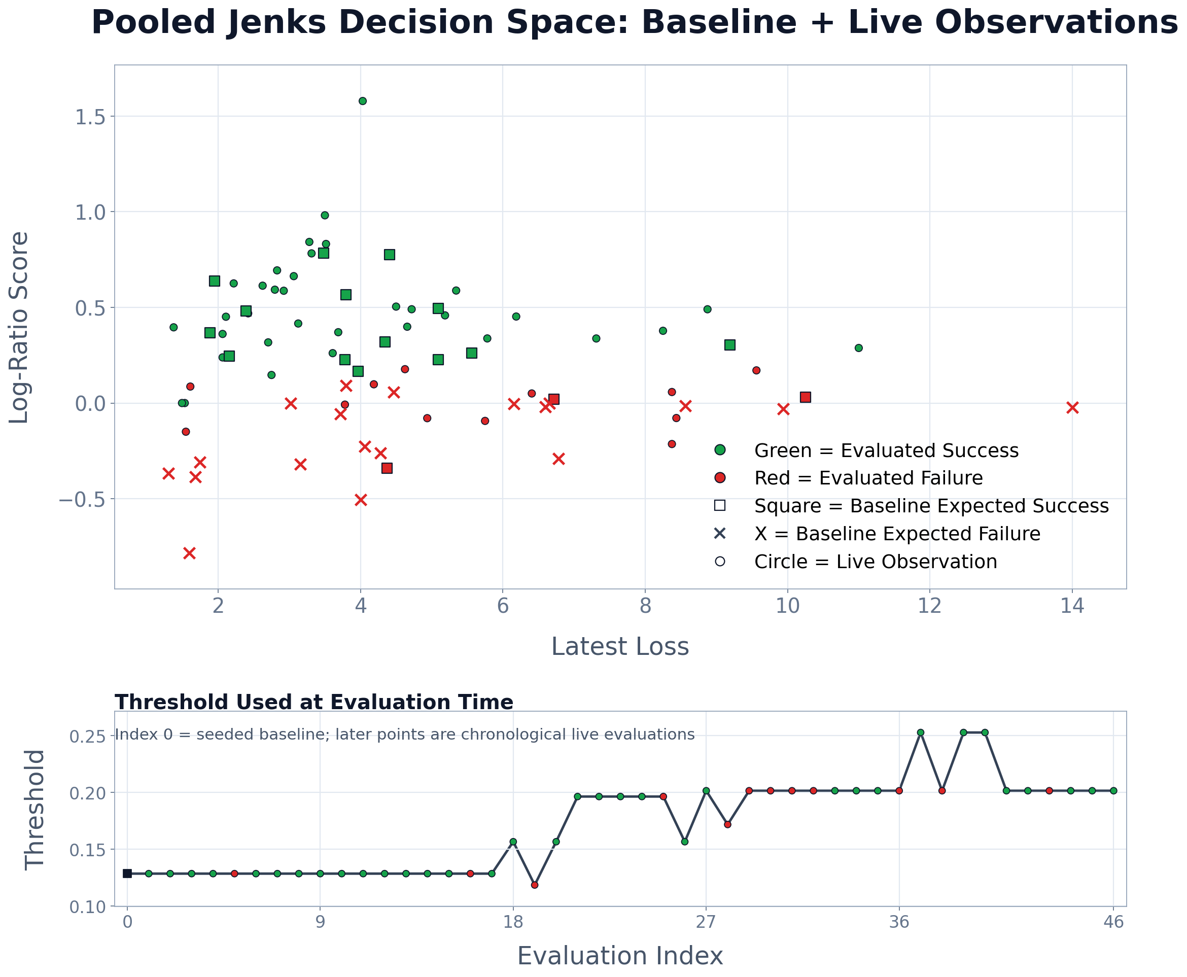
At runtime, TLv1 fits \(\kappa\) by pooling that seeded baseline with accumulated live observations and applying a two-class Jenks natural-break split over the log-ratio scores. The threshold therefore adapts to the observed score distribution while still starting from a concrete curated baseline rather than an empty history. Changes in \(\kappa\) do not trigger retroactive re-evaluation. That is, previously successful observations are retained even if they would fall below the updated threshold.
The seeded baseline, flattened loss tables, calibration figures, and interactive bundle are collected in the Equality Proxy artifact. For auditability, each observation record stores the underlying losses, the derived score \(r\), the margin relative to \(\kappa\), the threshold source and split statistics, the calibration sample count, and the exact scored prefixes and target text used in the decision.
Figure 1: Pooled decision space for TLv1’s loss-based agreement proxy. The top panel shows seeded baseline records together with live observations in latest-loss and log-ratio-score space, colored by evaluation outcome; the bottom panel shows the threshold used at evaluation time as the pooled score distribution evolves.
Observation Gating
Before the tutor-based score is allowed to decide promotion, TL applies a conservative precheck to ensure that the comparison record is reproducible and potentially discriminative:
Replayability and coverage: replay the previously successful observation computations and require the updated version to reproduce the retained shared evidence exactly, so its filtered successful-observation count is at least as large as the latest version’s.
Isolation: close/reload modules between runs so comparison between \(f\) and \(f'\) is not contaminated by state leakage.
Discriminating signal: require the observed computation to differ between latest and updated; otherwise there is no possible strict gain.
If any check fails, the ordinary observe path is aborted and does not count as a learning step. TLv1 may still permit progress through the branch-managing observe_branch path, which stages validated observations outside the main line until later merge conditions are met. These gates are intended to keep main-line learning steps consistent with the requirement that promotion witness \(T_{\Omega_E}(f') > T_{\Omega_E}(f)\).
Observation Outcomes
TLv1 exposes three evaluation outcomes:
observe: if the candidate passes, it immediately becomes the new incumbent theory.
observe_branch: if the candidate passes, it is promoted into a buffer namespace rather than main, without first satisfying the ordinary mainline replication/advantage gate. Buffered observations can accumulate and may merge back into main immediately once readiness checks pass. The buffer latest must still descend from the current main latest, pass replication against its own filtered successful-observation set, and strictly exceed main in filtered successful-observation count. Branch rewards are recorded as paused and released only for the merged lineage; residual paused rewards are cleared, as described in Reward states and release.
replace_observation: repairs failed replication items against the same archived (context, tutor_response) target. It is accepted only if latest still reproduces the archived original output exactly and the replacement from updated is not worse than the original by more than the calibrated margin. Successful replacements are staged on the updated version and enter the replication set only after a later successful observe.
Provenance and Reward
Runtime Traceability
The prototype traces compute dependencies at runtime with a multi-layer tracer centered on Python Enhancement Proposal (PEP) 669 (sys.monitoring) bytecode monitoring and supplemented by static analysis and a complementary sys.settrace tracer for cases that bytecode monitoring can miss. The goal is for the provenance DAG to track executed computation as closely as possible rather than rely only on static dependency estimates.
When knowledge or memory code runs, TL injects proxy objects such as knowledge, memory, conversation, tutor, and observe into the module namespace. Calls through these proxies are themselves recorded as provenance-tracked API results and registered immediately with the active tracer.
A compute call then records an explicit “used-to-produce” input set that includes the triggering conversation artifact, any proxy/API results consumed during execution, and the knowledge or memory definition artifacts (def_ids) actually read. If that compute result is returned into the dialogue, the conversation piece table stores the same def_id, preserving a direct link from the displayed output to its provenance lineage.
Step-Local Ancestry Graphs
On a successful observation, the system archives the evaluation record and builds a step-local ancestry graph rooted at the candidate-theory computation artifact. Concretely, this root is the def_id of the result of evaluating the observation expression under \(f'\). When that root belongs to the credited set, it serves as the credited root \(r\) for payout. The archived graph stores nodes, edges, and metadata including start_def_id.
Concrete archived ancestry graphs and reward slices can be inspected in the rewarded-observation artifacts, while lower-level dependency and piece-table examples are collected in the Benchmarks artifact. The next subsection describes the payout rule applied on this archived ancestry.
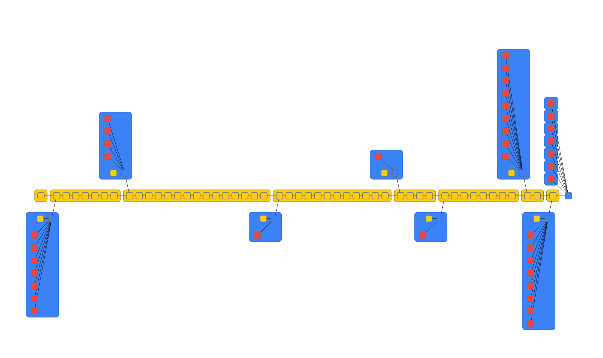
Figure 2: Representative first payout-step ancestry slice from rewarded Observation 1. The successful rooted computation appears in blue, the first payout recipient group in gold, and the immediate upstream edit definitions in red, showing the local rewarded slice from which payout begins.
For the full observation record, archived ancestry graph, and reward trace behind Figure 2, see Observation 1. Alternatively, for a more detailed walkthrough of the payout process, see Appendix D.
TLv1 Payout Rule
The Theory section presents, what I believe to be, a cleaner payout algorithm. TLv1 uses a different artifact/boundary/partition rule on the ancestry graph of each credited root.
As in Theory, fix a credited root \(r\). In TLv1, tracing used-to-produce edges backward from \(r\) yields an archived ancestry slice \(G_r\), which is the implementation-side counterpart of the Theory-side credited-root provenance DAG \(G=(V,E_G)\). Within \(G_r\), upstream llm_output artifacts attributable to \(c\) are absorbing; only these can retain reward. Non-absorbing artifacts matter only when they lie on some provenance path from an absorbing artifact to the current root; these are the rewardable non-absorbing artifacts. An eligible artifact is a rewardable non-absorbing artifact, other than the current root, with at least one rewardable non-absorbing parent.
The payout logic used in training TLv1 defines the local recipient set in three steps.
It defines continuation boundaries. Rewardable non-absorbing direct parents of the current root are root-local continuation roots: they mark the edge of the current payout call and become new roots when recursion continues. Other eligible artifacts that are first encountered when moving from an absorbing artifact toward the current root are first-hit boundaries. Root-local continuation roots recurse directly. First-hit boundaries pass their share uniformly to their rewardable direct parents, and those parents become the next payout roots.
It constructs a truncated local slice for the current payout call by reverse traversal over the rewardable ancestry from the current root, including boundary artifacts in the slice but not traversing past them within that call.
It then partitions the retained absorbing llm_output artifacts in that truncated slice into one or more local quotient groups. New boundary interfaces can split the same local slice into multiple absorbing groups.
The local recipient set consists of the absorbing quotient groups together with the root-local continuation roots and first-hit boundary artifacts.
Each payout call divides its incoming reward uniformly across that local recipient set. Absorbing groups retain their share locally. If multiple transfers target the same next root, their shares are added before the next recursive call.
PAYOUT(root, reward):
  groups, local_roots, first_hit_boundaries = EXTRACT_LOCAL_RECIPIENTS(root)
  recipient_count = |groups| + |local_roots| + |first_hit_boundaries|
  if recipient_count = 0:
    RECORD_ANOMALY(root, reward)
    return

  share = reward / recipient_count
  pending = {}

  for g in groups:
    omega_group[g] += share

  for u in local_roots:
    pending[u] += share

  for b in first_hit_boundaries:
    U = REWARDABLE_DIRECT_PARENTS(b)
    if U is empty:
      RECORD_ANOMALY(b, share)
      continue
    for u in U:
      pending[u] += share / |U|

  for u, reward_u in pending.items():
    PAYOUT(u, reward_u)
After recursion terminates, each absorbing-group weight is expanded uniformly across its member llm_output artifacts, additively across recursive paths and branches. The resulting per-output entries may be filtered by a minimum-reward threshold and consumed in training jobs. Empty-recipient calls and empty parent-routing sets are treated as anomaly states and are expected to be absent in normal runs.
Comparison note. On the 32 rewarded live observations, the theory-defined payout algorithm yields lower concentration than the archived TLv1 rule (gini: 0.663903 -> 0.529296; normalized_hhi: 0.005728 -> 0.001654; top_1_share: 0.033129 -> 0.010998). Total shifted mass is 12.3411 (mean 0.3857, median 0.3646 per observation), with a maximum of 0.66745 on obs_03-16_10-43-46-930851 and a minimum of 0.26105 on obs_03-16_11-26-48-115363.
Reward States and Release
A successful mainline observe produces immediately trainable pending_reward weights on llm_output artifacts. A successful observe_branch instead records pending_reward_paused, which becomes trainable only if a later branch merge succeeds.
At the payout boundary, terminal absorbing-group weights are expanded to per-llm_output weights, uniformly within each group and additively across branches, and written onto ancestry nodes as pending_reward or pending_reward_paused. For unmerged branch observations, later merge-time processing moves the paused entries to pending_reward and rescales them by the branch merge share. In this way, a single validated improvement yields both (i) an auditable record of what was compared and why it was accepted and (ii) concrete, reproducible weights on the specific llm_output artifacts that contributed to the success, with training eligibility determined by the reward state.
Offline Improvement of c
From Released Reward to Training Records
TLv1 does not update the refined heuristic function \(c\) online. Instead, it accumulates reward-weighted training records for later offline fine-tuning of the same policy. A local promotion under \(h\) establishes that a candidate edit to \(f\) was accepted on the current ledger, but only a record-setting promotion produces trainable pending_reward entries (see Reward states and release). Those released entries determine which earlier llm_output artifacts produced by \(c\) become weighted supervision targets.
Each invocation of the tool-augmented language model instantiating \(c\) is logged as an llm_output artifact containing the exact prompt/context, the sampled completion, and the call’s tracked I/O snapshot. After payout, released reward is written onto the corresponding llm_output nodes and aggregated by llm_output_def_id, producing weighted examples \((\text{prompt}_i, \text{completion}_i, w_i)\) with \(w_i \ge 0\) for later fine-tuning of \(c\). Branch-local entries in pending_reward_paused are excluded from the training set until the relevant branch is merged and the reward is released.
Reward-Weighted SFT Objective
TLv1 updates \(c\) with reward-weighted supervised fine-tuning rather than online reinforcement learning: completions that received more released credit contribute larger updates. In the simplest reward-weighted form, the objective is:
where \(\mathrm{CE}\) is token-level cross-entropy. The implemented TLv1 trainer uses a more explicit token-level form. If training example \(i\) has prompt/context \(p_i\), completion tokens \((z_{i,1}, \dots, z_{i,T_i})\), released reward \(w_i\), completion length \(T_i\), and reward-scale constant \(\alpha\), define
\[
a_i := \alpha \frac{w_i}{T_i}.
\]
For each completion-token position \(j \in \{1,\dots,T_i\}\), let
where \(\pi_{\mathrm{old}}\) is the logging policy that originally produced and logged the completion. In the clip_higher mode used for the TLv1 runs described here, the trainer applies ratio clipping with bounds \(\tau_{\mathrm{lo}}\) and \(\tau_{\mathrm{hi}}\) (default 0.8 and 1.28) and uses the surrogate loss
This keeps updates conservative by capping how far the current policy can increase the probability of rewarded logged tokens in a single update. The trainer also supports a reference-anchored Kullback-Leibler (KL) regularizer as an alternative mode, but that was not the stabilizer used in the runs discussed here.
Thus, rewarded improvements in \(f\) determine which earlier outputs of \(c\) count as useful, and those weighted outputs become the supervision signal for the next revision of \(c\).
Current Training and Serving Setup
In the current TLv1 runs, \(c\) is trained and served as a 4-bit-quantized GPT-OSS-20B base model plus a low-rank adaptation (LoRA) adapter checkpoint (rank \(r=8\), \(\alpha=16\)) learned offline from credited llm_output artifacts. Offline updates use reward-weighted LoRA SFT with the clip_higher stabilizer, bf16 training, and adamw_8bit, producing successive adapter checkpoints from the accumulated weighted dataset. At serving time, the UI loads the latest adapter on a single-GPU SageMaker endpoint (ml.g6e.xlarge) and enforces a 4600-token total context budget with a 600-token completion cap. For checkpoint history, dataset growth, and run-level recipe changes, see LoRA Training History.
Implementation Limitations
TLv1 has three main implementation limitations relative to the idealized formulation in the Theory section: imperfect provenance fidelity, use of a proxy evaluator for empirical agreement, and a remaining mismatch between the payout logic implemented in TLv1 and the cleaner rule presented there.
Provenance Fidelity Limits
TLv1 does not yet recover computation provenance with perfect granularity. Python bytecode optimizations and cases where runtime objects lack stable identity can obscure some fine-grained read/write dependencies. The prototype mitigates this with a multi-layer tracer built from PEP 669 sys.monitoring, static analysis, and a complementary sys.settrace path, and in the remaining edge cases falls back to conservative dependency heuristics when constructing edges for artifacts produced by executing heuristic-written theory or memory code.
The practical effect is usually coarser-than-ideal ancestry rather than missing ancestry altogether. Some edges are over-approximated, and some internal intermediates are collapsed into terminal outputs rather than represented as first-class provenance nodes. The targeted Benchmarks artifact and manual ancestry-graph audits suggest that the resulting graphs are broadly faithful to the underlying computations, but TLv1 still falls short of the provenance resolution assumed by the cleanest theoretical payout formulation. A lower-level runtime or more explicit execution model may eventually be needed to close that gap.
Evaluation-Proxy Limits
TLv1 operationalizes empirical agreement with a conditional-loss proxy rather than a direct agreement check on the observed target event. This choice makes the current implementation more flexible and appears to work in the initial 32-observation runs reported here, but its theoretical status remains unresolved. Because the deployed scorer is itself a stochastic language model, the evaluation rule introduces inductive structure that is not present in the minimal formulation developed in the Theory section.
The strongest mitigating consideration is that TLv1 uses the scorer only in a matched-pair comparison. For a given observation, the scorer, tutor target, committed pre-target context, committed computation expression, and prompt template are held fixed across the latest/updated comparison, and these shared elements all appear in the scored prefix. The only differential conditioning comes from the inserted computation result produced by latest rather than updated. Much of the scorer’s baseline preference for response format and surrounding context therefore cancels in the loss delta, so the comparison is driven more by the relative compatibility of the two candidate outputs with the same observed target under the same conditioning scaffold. Even so, the proxy remains a substantive approximation rather than a consequence derived from the theory itself.
Remaining Mismatch between TLv1 and the Cleaner Theory Formulation
TLv1 also still differs from the cleaner presentation in the Theory section. In particular, the payout logic used in the current implementation is not identical to the simpler rule proposed there. The results reported here were produced with the implemented TLv1 payout logic, while the Theory section presents a cleaner candidate replacement that I developed only after training had completed. I expect that further improvements to the payout logic, and a better theoretical justification of the payout structure, remain possible.
Conclusion
This essay proposes TL as a candidate physical formalization of scientific learning in a Critical Rationalist sense. It treats the learner as an embedded subsystem of the physical world and defines progress not by belief updates or fit to a fixed dataset, but by theory edits that survive explicit empirical comparison on a finite forward-chaining ledger built from an ordered stream of partial observations of world state.
This yields an architecture with an executable theory \(f\), improved by selection; a refinable heuristic function \(c\) that edits \(f\); an evaluator that promotes only validated improvements in empirical agreement; and a provenance system that traces successful outcomes back through the computational artifacts that helped produce them. When a proposed edit survives evaluation, the result is both a better current theory and a training signal for improving \(c\).
TLv1 is a first approximation to that theory. Its provenance tracking is still imperfect; its evaluator is a proxy whose theoretical status remains unresolved; and its payout logic is not derived from any strong theory of hierarchical computational provenance. Even so, the prototype shows that the full loop can be instantiated end to end. TLv1 learns by proposing theory edits, testing them against observations, selectively retaining theories of the physical world with greater empirical agreement, and converting successful learning steps into auditable credit assignments and offline updates to the refinable heuristic function \(c\) (e.g. the LLM), which serves as its current proposing policy.
If that loop continues to scale, the significance is broader than this prototype. It would suggest that possibly a major part of what is informally called scientific learning can be expressed as a concrete computational architecture rather than left at the level of informal description. Readers who want to inspect the current evidence can use the companion Artifacts page, which collects rewarded-observation bundles, equality-proxy calibration data, dependency-tracking benchmarks, and LoRA checkpoint history for the current 32 rewarded observations.
Appendix A: Conceptual Background
Embedded Learning Under Minimal Assumptions
Suppose science is a process that does or can occur in the physical world. With this framing, a definition of science falls in the domain of Physics (as opposed to pure Mathematics). The only world-level structure assumed here is an order/successor relation over the learner’s recorded observation stream, rather than a fundamental time parameter. In this paper, the index \(t\) simply labels this order: a learner can record transitions, and learning can be framed with respect to the resulting sequence. A minimally constrained definition of science would minimize extra assumptions about world dynamics (e.g., randomness).
Beyond grounding a formal definition of science in relation to a defined feature of the physical world, the remainder of the definition is guided by two proto-scientific frameworks.
Bayesian Confirmation Theory vs Critical Rationalism
Bayesian confirmation theory is a prominent approach to formalizing evidential support and theory comparison in the philosophy of science (Howson and Urbach 2006; Sprenger and Hartmann 2019). However, it remains in conflict with Critical Rationalism, a major competing framework that rejects treating uncertainty and belief updating as primitives. Critical Rationalism frames progress via conjecture and refutation (K. R. Popper 1963; Deutsch 2011). It emphasizes qualitative criteria for improvement, such as: a successor theory should be more precise and testable while extending explanatory scope; it should survive tests its predecessor fails; motivate and pass novel tests; unify previously unrelated problems; and be harder-to-vary (K. R. Popper 1963; Deutsch 2011). These ideas of Critical Rationalism have not yet been expressed in a coherent, formal (thus automatable) structure.
Separately, in machine learning pedagogy and practice, probability theory and Bayesian inference are often foregrounded (Goodfellow et al. 2016; Bishop 2006). Critical Rationalist critiques argue that probability theory cannot provide an inductive support relation of the kind to which Bayesian credences appeal. They further argue that stochastic components are explanatory commitments that should be introduced only when they play a necessary role in a particular theory (K. Popper and Miller 1983; K. R. Popper 1963; Deutsch 2012, 2016). These two frameworks of science remain in conflict. Neither has yet yielded an end-to-end computational formalism that reproduces the full set of desiderata of scientific progress when executed on a physical computer.
TL aligns with the Critical Rationalist framework, rejecting the treatment of uncertainty and belief updating as primitives. From its perspective, probability is an optional modeling commitment inside candidate theories, not a primitive of the learning rule. TL defines an agreement-based theory-selection algorithm anchored in an ordered stream of recorded observations.
Appendix B: Related Work
TL sits closest to neuro-symbolic systems, but it is also useful to compare it with broader systems that automate parts of hypothesis search, program induction, or scientific workflow. The most relevant comparison axes here are what counts as an observation, how symbolic hypotheses connect to raw inputs, how candidate changes are evaluated, and how accepted changes influence later proposal generation. The discussion below is representative rather than exhaustive and reflects the literature snapshot I had assembled by mid-2025 while developing the original “World Learning Algorithm” idea that later became TL.
Closest Related Work
The closest research neighborhood for TL is neuro-symbolic learning and reasoning (Garcez et al. 2009; Besold et al. 2017). WorldCoder is especially relevant because it uses an LLM to iteratively write and revise executable world-model code from interaction feedback (Tang, Key, et al. 2024). Related systems isolate parts of that loop. LLM-guided code repair ranks candidate programs by the fraction of tests or constraints satisfied (Tang, Hu, et al. 2024), while systems for inferring and revising natural-language rules through experimentation generate, test, and revise hypotheses (Piriyakulkij et al. 2024).
Within this neighborhood, the main differences from TL are fairly clear. Program-induction world-modeling systems such as WorldCoder usually work in structured simulated environments rather than over an ordered stream of partial physical-world observations (Tang, Key, et al. 2024). Other systems pair programmatic structure with learned perceptual or predictive components, as in programmatic video prediction (Tang et al. 2025). Some emphasize probabilistic evaluation of candidate models (Piriyakulkij et al. 2024; Curtis et al. 2025), while others emphasize compositional combinations of programmatic experts (Piriyakulkij et al. 2025).
Broader Adjacent Approaches
A looser but still relevant family includes self-improving coding agents and open-ended search methods. Some use quality-diversity search (Mouret and Clune 2015), while others use evolutionary selection over code or agent variants (Novikov et al. 2025; Zhang et al. 2025). These systems are relevant because they search over executable objects or improvement trajectories and can improve proposal quality over time, but in the forms cited here they are not framed around a fixed empirical promotion rule for replacing one world-theory with another.
Another adjacent line of work aims to automate parts of scientific practice at the workflow level by decomposing human-specified research goals into LLM-mediated hypothesis generation, critique, and ranking, as in an “AI co-scientist” (Gottweis et al. 2025). Such systems may accelerate components of existing scientific workflows, but the cited system is framed primarily as workflow assistance rather than as a general learning formalism specifying when one executable theory should replace another.
What TL Is Trying to Formalize
Relative to these efforts, TL differs mainly in what it tries to formalize. It does not start from a standard stochastic learning architecture and then add a scientific workflow layer or deductive constraints on top. Instead, it starts from a Critical Rationalist account of learning, treats the learner as physically embedded, and asks what minimal machinery is required for executable theories to be improved by empirical comparison on an ordered observation stream. That yields the specific formal package of a forward-chaining comparison ledger, an explicit promotion rule for theory selection, and a provenance-linked update path by which accepted improvements can later shape the proposal policy.
At the theory level, TL also tries to avoid building in strong assumptions about which features of the world are fundamental or whether stochastic structure must be taken as primitive. Probability may appear inside a candidate theory, but it is not part of the learning rule itself. TLv1, the current prototype, still uses approximations that are not derived cleanly from the full theory, as discussed in the main essay body. Even so, the distinctive ambition is not to retrofit an existing machine-learning architecture with more deductive or physically grounded language; it is to define scientific learning from first principles and then build the machinery implied by that definition.
Appendix C: Notation and Equations
This section collects the notation used throughout the essay, provides a rough mapping from symbols to concrete TLv1 artifacts, and summarizes the core equations used in the Theory section.
Notation
Term
Meaning
\(w\)
True world dynamics (the unknown function that updates the full world state)
\(t\)
Successor/order index (a label for the recorded observation sequence, not a metric time parameter)
\(k\)
Evaluation-step index used to refer to successive accepted evaluations
\(X_t\)
Full world state at index \(t\) (generally unobserved)
\(s\)
Observation interface (a sensor)
\(x_t\)
Partial observation at index \(t\)
\(x_i\)
\(i\)-th element of the evaluation window \(E\) (shorthand for some \(x_{t_i}\) in the global sensor stream)
\(E\)
Finite, sequence-ordered evaluation window of observed partial states \(x_t\)
\(I\)
Set of positions in \(E\) chosen as scored targets; each target position is later than every element of its conditioning tuple
\(g\)
Context-selection rule that maps each target position \(i \in I\) to an ordered conditioning tuple \(g(i)\) of earlier observations from \(E\)
\(\lambda\)
Ledger element in the fixed comparison ledger \(\Omega_E\)
\(\lambda_i\)
Newly committed ledger element associated with target position \(i \in I\), with fixed target \(x(\lambda_i)=x_i\) and singleton admissible replay-context set \(\mathcal{C}(\lambda_i)=\{g(i)\}\)
\(x(\lambda)\)
Fixed target observation associated with ledger element \(\lambda\)
\(\mathcal{C}(\lambda)\)
Admissible replay-context set associated with ledger element \(\lambda\)
\(\gamma\)
Generic admissible replay context ranging over \(\mathcal{C}(\lambda)\) in the agreement score definition
\(\Omega_E^{\mathrm{old}}\)
Previously validated ledger elements retained from earlier successful promotions because the current incumbent still succeeds on them under admissible replay
\(\Omega_E^{\mathrm{new}}\)
Newly committed forward-chaining instances derived from the current evaluation window \(E\)
\(\Omega_E\)
Fixed comparison ledger induced by evaluation window \(E\): retained prior validated elements together with newly committed forward-chaining instances from \(E\)
\(\mathcal{F}_E\)
\(\sigma\)-algebra on \(\Omega_E\) (here \(\mathcal{F}_E = 2^{\Omega_E}\))
\(\mu_E\)
Counting measure on \((\Omega_E, \mathcal{F}_E)\)
\(f\)
Executable theory function
\(f'\)
Candidate update to \(f\)
\(\tilde f\)
Generic previously promoted theory ranging over \(\mathcal{H}_{\mathrm{prom}}\) when defining \(T_{\Omega_E}^{\max}\)
\(F\)
Pairwise candidate set \(\{f, f'\}\) for a single evaluation step
\(T_{\Omega_E}(f)\)
Empirical agreement measure of \(f\) on the fixed comparison ledger \(\Omega_E\)
\(\mathrm{Eq}\)
Abstract equivalence relation on observations used in Theory
\(\widehat{\mathrm{Eq}}\)
Fixed, domain-agnostic proxy predicate used to approximate equivalence of observations
\(h\)
Theory evaluator (gates local promotions)
\(\text{success}(\Omega_E, f', f)\)
Promotion indicator on the fixed comparison ledger \(\Omega_E\)
\(c\)
Refined heuristic function (proposes theory updates and evaluations)
\(\mathcal{H}_{\mathrm{prom}}\)
Set of previously promoted theories
\(T_{\Omega_E}^{\max}\)
Best prior agreement score on the current ledger among theories in \(\mathcal{H}_{\mathrm{prom}}\)
\(\mathcal{N}(f,f')\)
Step-local root set associated with target events validated by the accepted promotion \(f \mapsto f'\)
\(\mathcal{R}\)
Credited root set at a reward event: roots whose validated target events account for the increment beyond the previous record
\(R\)
Reward-event indicator, with \(R=1\) exactly when a newly accepted theory sets a strict new record on the current ledger
\(R_r\)
Per-root reward share (uniform split of unit reward across \(r \in \mathcal{R}\))
\(r\)
Credited root artifact used as the payout root at a reward event
\(\mathcal{G}^{a}=(V^{a},E^{a})\)
Global provenance DAG at artifact granularity
\(\operatorname{AttrToC}(v)\)
Predicate indicating that artifact \(v\) is directly attributable to the refined heuristic function \(c\) and is eligible to receive terminal reward
\(G=(V,E_G)\)
Provenance DAG of the payout root used by the proposed payout rule (for the initial call, the credited root \(r\))
\(A_G\)
Absorbing artifacts in \(G\): artifacts directly attributable to \(c\) that may retain reward
\(V_r^{\mathrm{rel}}\)
Payout-relevant artifacts for root \(r\): artifacts lying on some provenance path from an absorbing artifact to \(r\); recursive calls reuse the same construction with \(q\) substituted for \(r\)
\(P(v)\)
Relevant parent artifacts of \(v\) within the rooted relevant-ancestry set (for the initial call, within \(V_r^{\mathrm{rel}}\))
\(\operatorname{ord}(v)\)
Sequence order of artifact \(v\) induced by its stable sequence identifier
\(S(r)\)
Spine of root \(r\) obtained by sequence-order backtracking
\(A(r)\)
Absorbing artifacts on the spine \(S(r)\)
\(B(r)\)
Relevant parent artifacts attached to the spine but not contained in it
\(\Gamma(r)\)
Recipient artifact set \(\Gamma(r)=A(r)\cup B(r)\); recursive calls use \(\Gamma(q)\) defined analogously
\(R_{\mathrm{in}}(q)\)
Reward entering the payout call rooted at \(q\); for an initial credited-root call, \(R_{\mathrm{in}}(r)=R_r\)
\(\sigma(q)\)
Per-artifact payout share at root \(q\), defined when \(\Gamma(q)\neq\varnothing\) by \(R_{\mathrm{in}}(q)/|\Gamma(q)|\)
\(W_q(a)\)
Total terminal reward assigned to absorbing artifact \(a \in A_G\) by the payout call rooted at \(q\); in particular, \(W_r(a)\) is the terminal reward distribution from credited root \(r\)
\(A_r^{\star}\)
Terminal absorbing artifacts in \(A_G\) that receive positive terminal weight under recursive payout from root \(r\)
\(\omega_r(a)\)
Per-root terminal weight contribution for root \(r\), with \(\omega_r(a)=W_r(a)\)
\(\omega(a)\)
Aggregated terminal weight assigned to absorbing artifact \(a\) across credited roots
\(\rho(a)\)
Abstract update record for absorbing artifact \(a\) (the logged local information used by the update rule to reinforce the choice by \(c\) that produced \(a\))
\(\mathcal{D}_r\)
Per-root weighted update record set: \(\mathcal{D}_r=\{(a,\rho(a),\omega_r(a)) : a \in A_r^{\star}\}\)
Updated \(c\) produced by applying the abstract update rule to \(c\) (e.g., offline training on weighted records)
artifact (ID)
Finest provenance-tracked unit (vertex in \(\mathcal{G}^{a}\)): stable identifier for an external input, output attributable to \(c\), tool result, or compute result
Throughout, agreement evaluation is forward-chaining: for each scored target position \(i \in I\), predictions may condition on any ordered tuple drawn from earlier observations \(\{x_j \in E : j < i\}\) and are scored once against the later target \(x_i \in E\).
Notation-to-TLv1 Mapping
In TLv1, the main Theory objects map to the following runtime components and persisted artifacts. The table is selective: it highlights the implementation correspondences most useful for reading the rest of the essay.
Formal object
TLv1 runtime component(s)
Primary persisted artifacts
\(f\) (theory)
Current promoted theory version (latest) executed via the knowledge API
Versioned theory text, piece-table lineage, and version metadata
\(f'\) (candidate theory)
Candidate theory version (updated) staged under the same versioned knowledge API until promotion
Candidate theory text and lineage artifacts staged for evaluation
\(c\) (refined heuristic function)
Tool-augmented language-model policy + API routing
llm_output I/O snapshots and llm_output definition artifacts
Committed evaluation record: \(E\) is the fixed observation window, while \(g(i)\) is operationalized by the committed pre-target context together with the committed computation expression and scoring prefix
Observation summaries storing the committed evaluation record and scoring metadata
Approximate TLv1 counterparts realized by local recipient extraction, boundary handling, quotient grouping, and recursive reward allocation on the archived ancestry graph
Derived payout structure computed from the archived ancestry graph
Reward-to-training-data pipeline: expand terminal weights to per-llm_output reward entries, then join those entries to recorded I/O snapshots and aggregate weighted training records
pending_reward / pending_reward_paused entries joined to llm_output snapshots and aggregated into weighted training records
\(c^{+}\) (updated heuristic function)
Offline-trained successor policy / adapter checkpoint
Reward-weighted SFT checkpoints and training-history artifacts
These correspondences are semantic rather than schema-exact; concrete file layouts remain implementation details.
Core Equations
The equations below are grouped by role: ledger construction, promotion and reward release, and provenance-based updating of \(c\). For recursive payout calls rooted at a boundary artifact \(q\), reuse the same rooted constructions with \(q\) substituted for \(r\) throughout: form the analogous relevant ancestry, parent relation, spine \(S(q)\), absorbing set \(A(q)\), boundary set \(B(q)\), and recipient set \(\Gamma(q)\) before applying the payout equations at \(q\).
Here \(\mathcal{R}\subseteq\mathcal{N}(f,f')\) denotes the credited roots whose validated target events account for the increment beyond the previous record \(T_{\Omega_E}^{\max}\) on the current ledger.
\[
\begin{aligned}
G &= (V,E_G) \\\\
A_G &= \{\, a \in V \mid \operatorname{AttrToC}(a)=1 \,\} \\\\
V_r^{\mathrm{rel}} &= \{\, v \in V \mid \exists a \in A_G \text{ such that } a \to^{*} v \to^{*} r \,\} \\\\
P(v) &= \{\, u \in V_r^{\mathrm{rel}} \mid (u,v) \in E_G \,\} \\\\
v_0 &= r \\\\
v_{i+1} &= \arg\max_{u \in P(v_i)} \operatorname{ord}(u) \qquad (P(v_i)\neq\varnothing) \\\\
S(r) &= (v_k, \dots, v_0) \\\\
A(r) &= \{\, s \in S(r) \mid \operatorname{AttrToC}(s)=1 \,\} \\\\
B(r) &= \left(\bigcup_{s \in S(r)} P(s)\right) \setminus S(r) \\\\
\Gamma(r) &= A(r) \cup B(r) \\\\
\sigma(q) &= \frac{R_{\mathrm{in}}(q)}{|\Gamma(q)|} \qquad (\Gamma(q)\neq\varnothing) \\\\
R_{\mathrm{in}}(u) &:= \sigma(q) \qquad (u \in \Gamma(q),\ \operatorname{AttrToC}(u)=0) \\\\
W_q(a) &=
\sum_{u \in \Gamma(q)}
\begin{cases}
\sigma(q) & \text{if } u = a \text{ and } \operatorname{AttrToC}(u)=1, \\\\
W_u(a) & \text{if } \operatorname{AttrToC}(u)=0, \\\\
0 & \text{otherwise,}
\end{cases} \\\\
A_r^{\star} &= \{\, a \in A_G \mid W_r(a) > 0 \,\} \\\\
\mathcal{D}_r &= \left\{\, \left(a,\rho(a),W_r(a)\right) : a \in A_r^{\star} \,\right\} \\\\
\mathcal{D} &= \left\{\, \left(a,\rho(a), \sum_{r' \in \mathcal{R}} W_{r'}(a)\right) : a \in \bigcup_{r\in\mathcal{R}} A_r^{\star} \,\right\} \\\\
c^{+} &= \operatorname{Update}(c;\mathcal{D}) \\\\
\end{aligned}
\]
Appendix D: Credit Assignment in TLv1
This appendix sketches TLv1’s implemented reward-distribution rule and gives one worked slice example.
Implementation sketch. In TLv1, reward distribution over a successful observation proceeds in five steps:
The runtime loads the archived nodes/edges for the observation’s ancestry graph into a dependency-graph view.
At each payout root, it computes a local recipient set with compute_recipient_nodes_for_dependency_graph. That set contains absorbing quotient groups, root-local continuation roots, and first-hit boundary artifacts.
Incoming reward is split uniformly across that local recipient set. Root-local continuation roots recurse directly; first-hit boundary artifacts first pass their share uniformly to their rewardable non-absorbing direct parents, and recursion continues from those parents.
Terminal quotient-group weights are expanded to per-llm_output weights and written to pending_reward or, for unmerged branch observations, pending_reward_paused.
On branch merge, only the merged branch observations’ paused rewards are released into pending_reward, scaled by the merge share; residual paused rewards in the buffer tree are cleared.
Empty local recipient sets, or first-hit boundaries with no rewardable parent set, are treated as anomalous states. TLv1 monitors for these conditions; they should not occur in normal operation, and they did not occur during live training.
Worked slice example.Figure 3 shows a step-local payout slice. The credited root r is the observed computation result of an updated knowledge version. At the first payout call, reward arriving at r is split uniformly across the local recipient set extracted at that root. In this slice, a_1, a_2, and a_3 are absorbing quotient groups that retain their local shares, while i_1, i_2, and i_3 are recursive boundary recipients that route reward onward. The lower boundary-expanded view spells out the routed branch beneath i_3, showing one concrete branch through which recursion continues.
The figure shows partitioned artifacts, including absorbing quotient groups and recursive boundary recipients (root-local and first-hit nodes). Ineligible artifacts are omitted. Credit is computed on the full archived graph; the diagram is an aggregated view of the relevant slice.
One interaction pattern underlying the schematic is:
a_1 (single llm_output): request a memory computation for the next curriculum topic; i_1 is the returned topic record used downstream.
a_2 (single llm_output): query the current theory through the knowledge API for a relevant definition; i_2 is the retrieved content used as an edit target.
a_3 (llm_output group): ask the tutor for guidance, edit the candidate theory version, and trigger an observation; i_3 is the updated theory definition written to the piece table.
r: the updated computation result for the observation (the credited root).
Boundary expansion is recursive and role-sensitive. For brevity, the figure spells out only one recursive branch: the one beneath i_3. Total reward is conserved throughout this routing. Shares assigned to absorbing groups terminate locally. The share assigned to a boundary branch is routed onward to its recipient set, and recursion continues from the resulting next payout roots. In this example, i_3 receives 1/6 of the reward assigned to r; after boundary expansion, the next payout call splits that share into 1/(6*5) portions. More generally, root-local continuation roots recurse directly, while first-hit boundaries route their share through rewardable direct parents before recursion continues.
Quotient groups can bundle multiple absorbing artifacts. In the quotient view, a_3 aggregates several adjacent llm_output artifacts because the intermediate tool calls do not introduce a new boundary crossing (e.g., they mostly write new state rather than reading an observed-theory boundary).
Example: underlying artifacts and quotient view (schematic)
The figure above is a quotient schematic; one concrete underlying artifact sequence (as stored in the conversation and logged API results) looks like this. This excerpt begins after a prior knowledge.create_version call has already produced candidate version 1, so the later edit and observe calls target that explicit updated version.
{"status":"success","result":{"index":0,"binding":"TOPIC_chem_density","title":"Chemistry: phase transitions and density","description":"Ice is less dense than liquid water (ice floats).","actions":[],"observation":{"computation":"","context":""},"completed":false},"expression":"get_next_topic()"}
[7] Theory content (recorded in executable theory version 1):
WATER = Substance(name="water", densities_kg_per_m3={"liquid": 1000.0, "solid": 917.0})
[8] LLM output (recorded in conversation):
{"assistant":{"api":"observe","action":"observe","params":{"version":1,"computation":"mass_of_volume(1.0, 'L', WATER, state='solid', mass_unit='kg')","context":"What is the mass (in kg) of 1.0 L of water in a solid state?"}}}
[9] API output (evaluated):
{"status":"success","observation_id":"obs_04-09_13-22-10","computation_observed":true,"sensor_data":["1.0 L of water weighs 0.92 kg."],"computation_outputs":{"latest":{"output":1.0},"updated":{"output":0.917}},"promoted_version":1}
Three concrete clarifications help interpret these quotient roles:
i_1 is a first-hit boundary because the memory.compute result in [2] depends on eligible non-absorbing memory-file artifacts, in this case get_next_topic() and/or the selected TOPIC_chem_density object. The API output is therefore the first conversation artifact on that branch whose parent set reaches into rewardable memory-file history.
i_2 is analogous on the theory side. The knowledge.find_node result in [4] depends on the latest-version WATER definition, which is an eligible non-absorbing knowledge artifact, so [4] becomes the first-hit boundary for that branch. Later, [6] writes a new WATER definition into candidate version 1, so the updated theory artifact grouped under i_3 has a different eligible artifact ID from the one underlying i_2.
The tutor response elicited by [5], not [5] itself, is the omitted external artifact here. [5] remains part of the absorbing group a_3. The returned tutor text is tracked as sensor_data and preserved in the full observation record, but it is not an eligible artifact because the runtime cannot record an internal provenance edge from the tutor.send request to the tutor text returned across the sensor boundary. In this example, that sensor artifact therefore does not become a rewardable path element.
The same logic also permits seeded memory or theory content. Executable files may contain artifacts not written by the model; if those seeded artifacts have no upstream path to absorbing llm_output nodes, they can influence computation but remain ineligible for reward flow. More generally, credit flows only through artifacts that both enter the archived ancestry slice and connect back to absorbing llm_output history.
References
Besold, Tarek R., Artur d’Avila Garcez, Sebastian Bader, et al. 2017. “Neural-Symbolic Learning and Reasoning: A Survey and Interpretation.”arXiv Preprint arXiv:1711.03902, ahead of print. https://doi.org/10.48550/arXiv.1711.03902.
Bishop, Christopher M. 2006. Pattern Recognition and Machine Learning. Information Science and Statistics. Springer.
Curtis, Aidan, Hao Tang, Thiago Veloso, et al. 2025. “LLM-Guided Probabilistic Program Induction for POMDP Model Estimation.”Proceedings of the 9th Conference on Robot Learning, Proceedings of machine learning research, vol. 305: 3137–84. https://proceedings.mlr.press/v305/curtis25a.html.
Deutsch, David. 1985. “Quantum Theory, the Church-Turing Principle and the Universal Quantum Computer.”Proceedings of the Royal Society of London A: Mathematical and Physical Sciences 400 (1818): 97–117. https://doi.org/10.1098/rspa.1985.0070.
Deutsch, David. 2011. The Beginning of Infinity: Explanations That Transform the World. Penguin.
Deutsch, David. 2016. “The Logic of Experimental Tests, Particularly of Everettian Quantum Theory.”Studies in History and Philosophy of Science Part B: Studies in History and Philosophy of Modern Physics 55: 24–33. https://doi.org/10.1016/j.shpsb.2016.06.001.
Gottweis, Juraj, Wei-Hung Weng, Alexander Daryin, et al. 2025. “Towards an AI Co-Scientist.”arXiv Preprint arXiv:2502.18864, ahead of print. https://doi.org/10.48550/arXiv.2502.18864.
Howson, Colin, and Peter Urbach. 2006. Scientific Reasoning: The Bayesian Approach. 3rd ed. Open Court.
Mouret, Jean-Baptiste, and Jeff Clune. 2015. “Illuminating Search Spaces by Mapping Elites.”arXiv Preprint arXiv:1504.04909, ahead of print. https://doi.org/10.48550/arXiv.1504.04909.
Novikov, Alexander, Ngân Vũ, Marvin Eisenberger, et al. 2025. “AlphaEvolve: A Coding Agent for Scientific and Algorithmic Discovery.”arXiv Preprint arXiv:2506.13131, ahead of print. https://doi.org/10.48550/arXiv.2506.13131.
Piriyakulkij, Wasu Top, Cassidy Langenfeld, Tuan Anh Le, and Kevin Ellis. 2024. “Doing Experiments and Revising Rules with Natural Language and Probabilistic Reasoning.”Advances in Neural Information Processing Systems 37. https://doi.org/10.48550/arXiv.2402.06025.
Piriyakulkij, Wasu Top, Yichao Liang, Hao Tang, Adrian Weller, Marta Kryven, and Kevin Ellis. 2025. “PoE-World: Compositional World Modeling with Products of Programmatic Experts.”arXiv Preprint arXiv:2505.10819, ahead of print. https://doi.org/10.48550/arXiv.2505.10819.
Popper, Karl R. 1963. Conjectures and Refutations: The Growth of Scientific Knowledge. Routledge & Kegan Paul.
Popper, Karl, and David Miller. 1983. “A Proof of the Impossibility of Inductive Probability.”Nature 302: 687–88. https://doi.org/10.1038/302687a0.
Sprenger, Jan, and Stephan Hartmann. 2019. Bayesian Philosophy of Science. Oxford University Press.
Tang, Hao, Kevin Ellis, Suhas Lohit, Michael J. Jones, and Moitreya Chatterjee. 2025. “Programmatic Video Prediction Using Large Language Models.”arXiv Preprint arXiv:2505.14948, ahead of print. https://doi.org/10.48550/arXiv.2505.14948.
Tang, Hao, Keya Hu, Jin Peng Zhou, et al. 2024. “Code Repair with LLMs Gives an Exploration-Exploitation Tradeoff.”Advances in Neural Information Processing Systems 37. https://doi.org/10.48550/arXiv.2405.17503.
Tang, Hao, Darren Key, and Kevin Ellis. 2024. “WorldCoder, a Model-Based LLM Agent: Building World Models by Writing Code and Interacting with the Environment.”Advances in Neural Information Processing Systems 37. https://doi.org/10.48550/arXiv.2402.12275.
Zhang, Jenny, Shengran Hu, Cong Lu, Robert Lange, and Jeff Clune. 2025. “Darwin gödel Machine: Open-Ended Evolution of Self-Improving Agents.”arXiv Preprint arXiv:2505.22954, ahead of print. https://doi.org/10.48550/arXiv.2505.22954.